Modeling the Heapsort Algorithm in Alloy

Heapsort is a fundamental sorting algorithm with O(nlogn) time complexity. It is based on transforming a given unsorted array into a binary tree (a heap) and recursively operating over its nodes to incrementally come up with the sorted version of the original array. In this post, I attempt to prove its correctness, i.e., the postcondition arr[i] >= arr[j] for any given indices i, j such that i>j. For simplicity, I am only concerned with sorting integer arrays in ascending order. And, for the proof, I use Alloy, a software modeling and verification tool with a declarative modeling language that combines first-order logic and relational calculus ¹.

My ultimate goal is to utilize Alloy for reasoning about more intricate graph algorithms I devised in a climate modeling configuration tool, which is the subject of a future post. Hopefully, this post serves as an exercise for myself on how state-based formalism can be employed to reason about the correctness of algorithms that operate on data structures like trees and graphs recursively.

Before delving into its verification model, I describe the heapsort algorithm for those whose CS101 memory is rusty. Otherwise, you may skip the next section.

The heapsort algorithm

Here, I provide a quick overview of the algorithm along with a simple Python implementation. More in-depth description and analysis may be found in introductory algorithms textbooks, such as the popular CSLR² book.

Figure 1: The heapsort algorithm. (wikimedia, RolandH)

The first step of the heapsort algorithm is to transform the original array into a heap representation, i.e., an ordered binary tree. In the context of array sorting, we specifically make use of max-heaps, i.e., heaps with nodes that have values greater than the values of its two child nodes (left and right). Below is an example max-heap where you can observe this property.

Figure 2: An example max-heap representation (wikimedia, Kelott)

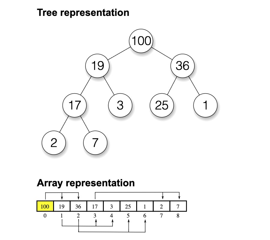Also, in the above array representation with zero-based indexing, observe the following relations between the indices of the i.th node and its two children:

• If exists, the index of its left child is 2*i+1.
• If exists, the index of its right child is 2*i+2.

Or, in Python:

def left(i):
    return 2 * i + 1
def right(i):
    return 2 * i + 2

To impose the max-heap property, i.e., the condition that the values of parent nodes are greater than those of their children, we define a recursive function that traverses the nodes of array a (of type numpy array) in a downward fashion.

def max_heapify(a, i, heap_size):
    """Starting from the i.th node, apply the max-heap
    property along a branch until a leaf node or a node
    that satisfies the max-heap property is encountered.
    """
    l = left(i)
    r = right(i)
    if r < heap_size and a[r] > a[i] and a[r] > a[l]:
        a[r], a[i] = a[i], a[r]
        max_heapify(a, r, heap_size)
    elif l < heap_size and a[l] > a[i]:
        a[l], a[i] = a[i], a[l]
        max_heapify(a, l, heap_size)
    else:
        return

Although recursive, the max_heapify function imposes the max heap property locally along a single branch until a leaf node or a node that already satisfies the max-heap property is encountered. To transform an entire array into a max-heap then, below is a function that calls max_heapify repeatedly:

def build_max_heap(a):
    """Calls max_heapify for non-leaf nodes.
    Starts from lower branches and moves
    upwards to the root node."""
    for i in range(len(a)//2-1, -1, -1):
        max_heapify(a,i,len(a))

Notice in the above for-loop that we call max_heapify for the first half of the array a only, since the latter half corresponds to leaf nodes which trivially satisfy the max-heap property by definition. Having defined all of the necessary helper functions, below is the heapsort function that sorts a given unsorted array a.

def heapsort(a):
    heap_size = len(a)
    build_max_heap(a)
    for i in range(len(a)-1, 0, -1):
        a[0], a[i] = a[i], a[0]
        heap_size -= 1
        max_heapify(a,0,heap_size)

When we first call the build_max_heap function above, the largest value gets moved to the front of the array (i.e., a[0]). Subsequently, in the first step of the for-loop, the largest value gets moved to the end of the heap as a result of swapping a[0] and a[i]. We then decrement the heap_size and call max_heapify to move the next largest value to the front of the array again. We repeat the process for all i, i.e., until all values are ordered.

Alloy Analyzer

Alloy is a software modeling language and analyzer. Its declarative language combines first-order logic and relational calculus that enable developers to specify their software systems in an abstract but precise manner. So, the Alloy language is quite simplistic, minimalistic, and very high-level. As such, a typical Alloy model consists of a couple of hundred lines of code at most, however complex the actual software implementation may be. ³

Like other model checkers, and unlike theorem provers, the Alloy analyzer is an automated verification tool. Given an abstract representation, which is to be specified by the user in Alloy language, the analyzer generates all possible configurations, valuations, and execution traces within a bound and exhaustively searches for violations of structural and behavioral assertions, again, specified by the user. The exhaustive and automated nature of the search ensures that all possible corner cases are discovered regardless of how likely or unlikely they are in the real world. This assurance is the main advantage of formal methods over testing.

In the remainder of this post, I will briefly describe the Alloy language constructs and features as we encounter them in my Heapsort model. The descriptions will appear in text boxes like this one. Note, however, that this is by no means a complete introduction to Alloy. For those who’d like to learn more about the language and the tool, here is a highly recommended 8-minute video introduction by Daniel Jackson, the principal designer of Alloy: Alloy: Language Tool for Software Designs. And here is an online tutorial that covers the latest versions of the tool and the language: Alloy Tutorial.

Alloy Model of Heapsort

The first step of developing an Alloy model is to specify the structure of the system to be modeled. So, we begin by specifying a conceptual structure that represents arrays:

one sig Array {
  var values:  Int -> lone Int,
}

In Alloy, signatures are declared with the sig keyword and are used to specify conceptual structures and types. Similar to how classes in object oriented languages may contain data members and methods, signatures in Alloy may have fields. In the above declaration, the Array signature has a single field called values. Just like how the dot operator (.) is used in object oriented languages to access class members, the dot join operator (.) in Alloy may be used to access signature fields. For example, a.values returns the values field of an Array instance a.

The one keyword preceding the signature definition states that our model should have exactly one array instance. This is because we are not concerned with interactions between multiple arrays. Rather, we are concerned with how the ordering of the values of an arbitrary array gets changed by the heapsort algorithm.

In above Array signature definition, the values field is of type Int -> lone Int, i.e., a mapping from integers to integers. So this field may be thought of as binary relation from integers to integers where the domain (of type Int) corresponds to indices and the range (again, of type Int) corresponds to the values. By default, all Alloy relations are immutable. To state that the values field is mutable, we declare it with the var keyword, which is a new addition to the Alloy language. This enables us to modify the values field down the line via functions or predicates that describe the dynamic aspects of the model.

The arrow product operator -> is used to define relations. A relation definition P -> Q represents a set of tuples (p, q) for all p in P and for all q in Q where P and Q are sets. Multiplicity keywords such as lone, may be specified in a relation definition to bound the possible combinations of (p, q). For example, the lone multiplicity above ensures that each index can be mapped to at most one value. (However, a value may be shared by multiple indices.)

Instead of a binary relation values: Int -> lone Int, one might suggest simply defining the values field as a set of integers, e.g., values: Int. But the correctness property we aim to prove has to do with the relation between indices and values. Hence, the modeling decision to specify the values field as a binary relation and not a set of Integers. Yet it is still quite straightforward to access the value at the i.th element of an array instance a using the box join operator as follows: a.values[i]. Also, we can get the set of indices using the following let expression:

let indices[a] = (a.values).Int

let expressions allow modelers to define short references to long or complex expressions that may appear repeatedly in the model. A major language feature used in the above let expression is the dot join operator that joins a.values and Int (the set of all integers) to get their relational composition, which is simply the set of indices of a.

While at it, we can also define the following let expressions for computing the indices of child nodes of a node with index i, as well as a let expression that represents the length of a given array instance a:

let left[i] = (i.mul[2]).add[1]
let right[i] = (i.mul[2]).add[2]
let length[a] = max[indices[a]].add[1]

Notice above that we use add and mul functions for integer addition and multiplication. Similarly, we use sub and div for subtraction and division of integers. This is because the operators + and - are reserved for specifying set union and set difference.

Having defined the structure of our problem, we can execute this early version of the model in Alloy Analyzer. The following is a random model instance that is generated by Alloy:

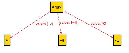
The above Array instance has three elements (-7, 4), (-4,-8), (0,-1) where the first and second items of the tuples correspond to indices and values, respectively. Upon quick inspection, it is apparent that the indices {-7, -4, 0} are faulty. They should instead be in sequential order starting from 0. ( We are assuming 0-based indexing). To enforce this structural rule, we declare the following fact, i.e., a global constraint to hold at all times.

fact{
  all a: Array | all i: indices[a] | 
    i.minus[1] in indices[a] or i=0
}

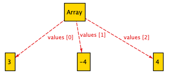
This fact definition states that for any given array a, and for any given index i of a, i-1 must also be an index of a. Otherwise, i must be 0. We confirm that this fact definition ensures valid indices by executing the model again and inspecting several randomly generated instances, one of which is shown below:

We are now ready to model the dynamic aspects of the heapsort algorithm. Recall from the previous section that one of the basic operations appearing in max_heapify and heapsort routines is swapping the values of two items in array a. We model this operation by defining the following Alloy function:

fun swap[values:Int->Int, i, j :Int] : Int->Int {
	values ++ ( i->values[j] + j->values[i] )
}

The swap function above makes use of the override operator ++, which is typically used for assignment-like statements and updating the entries in a relation.

Given a values field and two indices i and j, the above function returns a new values instance (of type Int->Int) where the values of i.th and j.th elements are swapped.

The next function models the recursive max_heapify routine:

fun max_heapify[values:Int->Int, i,heap_size:Int]:Int->Int{
    right[i] < heap_size and 
    values[right[i]] > values[i] and 
    values[right[i]] > values[left[i]]  implies
        max_heapify[
            swap[values, i, right[i]],
            right[i], 
            heap_size]
    else left[i] < heap_size and 
    values[left[i]] > values[i] implies
        max_heapify[
            swap[values, i, left[i]],
            left[i], 
            heap_size]
    else values
}

Similar to the original Python implementation, the max_heapify function above recursively applies the max-heap property along a branch starting from a given i.th node until a leaf node or a node that satisfies the max-heap property is encountered. As in the original implementation, the max_heapify function consists of three conditional branches. The first conditional branch is visited if the value of the right child is to be swapped with the parent, while the second conditional branch is visited if the value of the left child is to be swapped. Otherwise, the function returns the original values instance.

By default, Alloy doesn’t support recursive calls. But the restriction may be lifted by changing the Recursion Depth setting in the Options menu. Note, however, that a more Alloyesque way to specify recursive behavior is via the transitive closure operator.

The next routine to incorporate in the Alloy model is the build_max_heap function. This time, instead of a function, we choose to specify the routine as a predicate.

The main difference between functions and predicates is that functions return a value whereas predicates return true or false depending on whether they are feasible or not.

pred build_max_heap[a: Array]{
    some iter: Int->Int->Int {
        iter[(length[a].div[2]).add[1]] = a.values
        all i: indices[a] | i<= length[a].div[2] implies
            iter[i] = max_heapify[
                iter[i.add[1]],
                i,
                length[a]]
        a.values' = iter[0]
    }
}

Recall that the original build_max_heap function consists of a for-loop that iterates backward over non-leaf heap array nodes. As a declarative language, Alloy doesn’t have an equivalent of for-loops. While a quantification constraint may be used to represent loops with no loop dependence, incremental loops that exhibit stateful behavior are harder to represent in declarative languages. The for-loop in build_max_heap brings about one such complication since the order in which the max_heapify function gets called determines the correctness of the algorithm. This is called the incremental update problem.

In the above build_max_heap predicate definition, the incremental update problem is addressed by an approach that was introduced in a paper I co-authored ⁴. The approach is based on defining an iteration table iter which is indexed by an Int timestamp. While the first two columns of the iter table correspond to the values field of array a, the last column corresponds to an Int timestamp, which allows us the capture the stateful behavior since we can relate consecutive iterations of values by indexing the iter table. Since the original for-loop steps backward though, the final outcome of iteration is iter[0]. Thus, a.values' gets set to iter[0].

The latest version of Alloy (v.6) extends the language to express mutable signature and fields using the var keyword. The values field of Array signature is one such field. The value of a mutable field in the next state is denoted by the quote symbol ('), so a.values' expression in the build_max_heap predicate corresponds to the modified ordering of array elements as a result of executing the routine.

The final routine for specifying the dynamic behavior is the heapsort routine. In the heapsort specification below, we again make use of the quote operator (') to denote the incremental progression of the values field as the algorithm gets executed. So the three states of the values field are:

a.values	The initial (unsorted) state of the array values
a.values'	The intermediate state (after executing build_max_heap)
a.values''	The final state (after executing heapsort)

pred heapsort [a: Array] {
    build_max_heap[a]

    some iter: Int->Int->Int {
        iter.Int.Int =  a.values.Int +length[a] // timestamps

        iter[length[a]] = a.values'
        all i: indices[a] |
            let t = i, t_prev = i.add[1] |
            let swapped = swap[iter[t_prev], 0, i] |
            iter[t] = max_heapify[swapped, 0, i]

        a.values'' = iter[0]
    }   
}

Similar to the for-loop in build_max_heapify routine, the for-loop in heapsort routine is represented with an iteration table to account for stateful behavior. Right before the quantification constraint (all i: indices[a]) we set iter[length[a]] to be equal to a.values. Since the iteration is backwards from the last element of a to the first element, iter[length[a]] corresponds to the state before the iteration begins. And so iter[0] corresponds to the final state of values. Hence, a.values'' = iter[0] equality specification at the end of the heapsort predicate.

Analysis

Before analyzing the model, we restrict the model to have a small number of values in the spirit of the small scope hypothesis which is based on the idea that most bugs have small counterexamples, and, thus, an analysis that considers all small instances can reveal most flaws ³. So, we set the max number of values to 7, which is the largest 4-bit integer. (By default, Alloy considers 4-bit integers only.)

fact {
    all a: Array | #a.values <= 7
}

The correctness property that we aim to prove is that every execution of the heapsort algorithm results in sorted values. The following predicate checks whether a given value instance (of type Int->Int) is sorted:

pred sorted[values:Int->Int] {
    all i,j : values.Int | i<j implies values[i] <= values[j] 
}

Before checking the above property, let’s ask the Alloy analyzer to generate model instances for us to visually inspect:

pred show{
  all a: Array |  not sorted[a.values] and heapsort[a]
}

run show for 3 steps

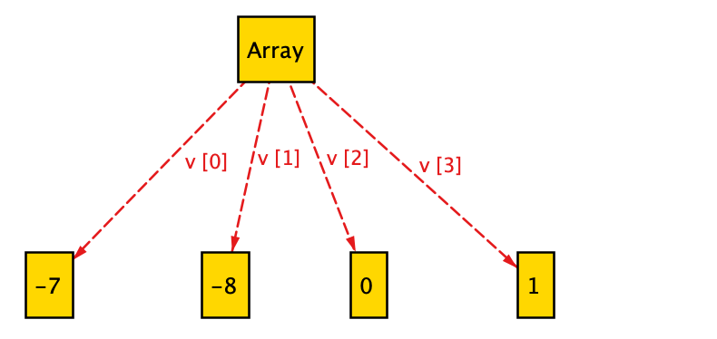
By executing the above run command for 3 steps, we get several arbitrary model instances, one of which is shown below. Note that the three states correspond to (1) the initial state, (2) the state after running build_max_heap and (3) the final state. Also note that the visualization theme is customized for brevity, e.g., by renaming values field as v.

(1) The initial, unsorted state:

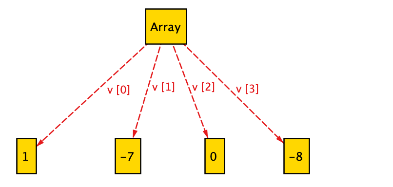
(2) The intermediate, max-heap state:

(3) The final, sorted state:

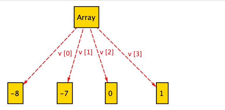
As seen in the final state above, the initially unsorted array gets sorted accurately. But the run command allows us to visually inspect only a few instances. To check that the property holds for all instances within the given bound, we execute the following check command:

assert is_sorted {
     all a:Array | heapsort[a] implies sorted[a.values'']
}

check is_sorted for 3 steps

The Alloy output confirms that no counterexample is found. Thus, we have proved that our heapsort specification successfully sorts any given array with a length less than or equal to 7.

Executing "Check is_sorted for 3 steps"
   Solver=minisat(jni) Steps=1..3 Bitwidth=4 MaxSeq=4 SkolemDepth=1 Symmetry=20 Mode=batch
   1..3 steps. 348351 vars. 26217 primary vars. 695094 clauses. 76908ms.
   No counterexample found. Assertion may be valid. 116759ms.

Remarks

Alloy, and formal methods in general, can be employed to quickly frame questions and get answers regarding the structure and behavior of software, regardless of how complex the actual system may be. In this post, I have presented a toy model but the application of formal methods is not limited to such hypothetical problems. An actual bug in the implementation of another sorting algorithm, TimSort (the main sorting algorithm in Java and Python), was found via formal methods. See link.

References

1. Jackson, Daniel. “Alloy: a language and tool for exploring software designs.” Communications of the ACM 62.9 (2019): 66-76. ↩

2. Cormen, Thomas H., et al. “Introduction to Algorithms. third edition.” New York (2009). ↩

3. Jackson, Daniel. Software Abstractions: logic, language, and analysis. MIT press, 2012. ↩ ↩²

4. Dyer, Tristan, Alper Altuntas, and John Baugh. “Bounded verification of sparse matrix computations.” 2019 IEEE/ACM 3rd International Workshop on Software Correctness for HPC Applications (Correctness). IEEE, 2019. ↩